In this first blog post, I would like to share my thoughts on how the Kriging method can often lead to confusion due to its different interpretations. My goal is to help readers distinguish between Kriging (the “Best Linear Unbiased Predictor (BLUP)”) viewed from the linear algebra perspective (as a solution of a linear system of equations) and its probabilistic interpretation as a Gaussian random field (the term “Gaussian process” I prefer using it for data without a spatial reference).
In Part 1, I will present the equations used to calculate the Kriging weights and demonstrate how to predict values at specific spatial locations. Using these weights, we will then perform interpolation over a regular square grid covering the entire spatial domain of interest. Finally, the results from our manual calculations will be compared with those obtained using the “gstat” package to assess their consistency and accuracy.
1 Introduction
We will denote the spatial locations as \(\{\mathbf{s}_1, \ldots, \mathbf{s}_n\}\), and the spatial data collected at these locations (the observed or measurement variable) will be denoted as \(Z(\mathbf{s}_1), \ldots, Z(\mathbf{s}_n)\). The spatial locations are determined by their coordinates in the space, for example, latitude-longitude and we will be mainly focused in the two-dimensional space. To denote the vector of all the observations we will use \(\mathbf{Z} = (Z(\mathbf{s}_1), \ldots, Z(\mathbf{s}_n))^{\top}\).
2 Computing the distance
Distance is a numerical description of how far apart things are. It is the most fundamental concept in geography. Considering the Waldo Tobler’s first law of the geography which says everything is related to everything else, but near things are more related than distant things (Tobler 1970) , we need to quantify this relationship in some way and it is not always as easy a question as it seems.
Computing the distance between a set of spatial data points is very important for spatial data analysis. If we have \(\mathbf{s}_i\) spatial locations, for \(i = 1, \ldots, n\), with \(n\) equal to the total number of spatial locations. The coordinates of \(\mathbf{s}_i\) are in latitude-longitude but for simplicity, we will denote them as \((x_i,y_i)\). Now, another set of spatial locations \(\mathbf{s}_j\) has coordinates \((x_i, y_j)\), hence the Euclidean distance between spatial points \(\mathbf{s}_i\) and \(\mathbf{s}_j\) is given by
There are other forms to calculate the distance, for example; great-circle distance, azimuth distance, travel distance from point to point, time needed to get from point to point, etc.).
The computation of “distances” are commonly represented by the distance matrix. In this object (the distance matrix) we have all the values calculated for the distances between the objects of interest. For example,
In simple terms, it is a function of difference over distance. In mathematical terms, we could define it as the expected squared difference between values separated by a distance vector, generally denoted as \(h\). The equation of the Variogram is the following
where \(\mathbf{s}\) is the spatial location, \(\mathbf{h}\) is the vector of distance between two spatial points, and \(\gamma(\mathbf{h})\) measured how dissimilar the field values become as \(\mathbf{h}\) increases (this is for a third type of stationarity (intrinsic stationarity) and assuming that \(\mathbb{E}[Z(\mathbf{s} + \mathbf{h}) - Z(\mathbf{s})] = 0\)). The relationship of the variogram and the covariance function is given by:
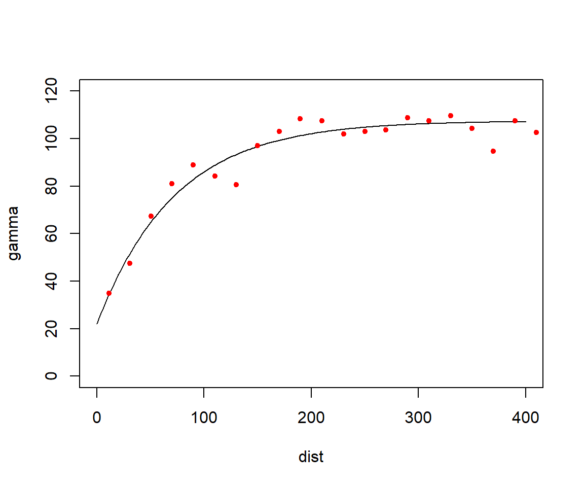
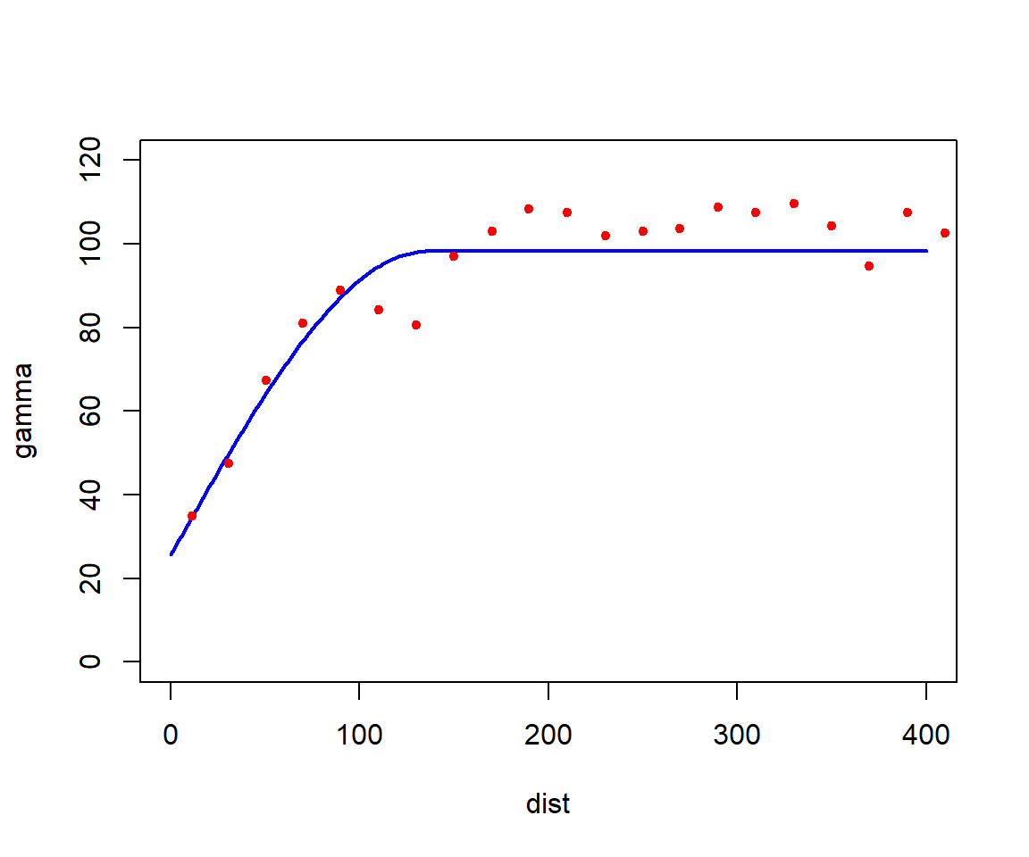
Traditionally, the selection of a variogram model begins with plotting the empirical semivariogram. This empirical plot is then visually compared against various theoretical models to identify the most appropriate fit. The standard form of the empirical semivariogram is given by
where \(Z(\mathbf{s}_i)\) and \(Z(\mathbf{s}_j)\) are the values (in the space) at the spatial locations \(\mathbf{s}\). Finally, we will denote the variogram as \(2 \gamma(\mathbf{h})\).
For all the variograms presented, \(\rho\) is the range parameter.
4 Variogram computation
From the Equation 4, we know that; \(n(\mathbf{h})\) is the number of spatial points for a specific distance vector \(\mathbf{h}\), with \(Z(\mathbf{s})\) and \(Z(\mathbf{s} + \mathbf{h})\) and \(2 \gamma(\mathbf{h})\) is the variogram.
First, we will consider the following important observations before of the computation:
As the distance increase, then the variability also increase: this is typical, as larger distance offsets generally lead to greater differences between the head and tail samples.
It is calculated over all possible pairs separated by the distance vector \(\mathbf{h}\): we evaluate all data, identifying all possible pair combinations with every other spatial point. The variogram is then calculated as half the expected squared difference between these pairs. A larger number of pairs provides a more reliable estimate.
It is necessary plot the sill to know the correlation between the spatial points: here, sill is the spatial variance \(\sigma^2_{\mathbf{s}}\). As we are assuming stationarity, the covariance is:
The covariance measure the similarity over distance, and if \(\sigma^2_{\mathbf{s}} = 1.0\), \(C(\mathbf{h})\) is equal to the correlogram \(\rho(\mathbf{h})\) such that:
The distance at which the variogram reaches \(\sigma^2_{\mathbf{s}}\) is known as the range: the distance in which the difference of the variogram from \(\sigma^2_{\mathbf{s}}\) becomes negligible.
Evaluate the discontinuity at the origin, the nugget effect: It represents variability in the data that occurs at scales smaller than the sampling distance, or it may be caused by measurement errors or random noise.
where \(n(\mathbf{h})\) is the number of pairs \((i, j)\) such that the distance between \(\mathbf{s}_i\) and \(\mathbf{s}_j\) is approximately \(\mathbf{h}\).
For \(\mathbf{h} = 2\), the pairs of points whose distance is 2 are:
\((\mathbf{s}_1, \mathbf{s}_2)\)
\((\mathbf{s}_2, \mathbf{s}_3)\)
\((\mathbf{s}_3, \mathbf{s}_4)\)
\((\mathbf{s}_4, \mathbf{s}_5)\)
We now calculate the squared differences for each pair of spatial points:
Thus, for \(\mathbf{h} = 2\) is \(\hat{\gamma}(2) = 1.625\).
4.2 Using the “gstat” package of R
The “gstat” package in R is a versatile tool used for geostatistical modelling, spatial prediction, and multivariable geostatistics (Pebesma 2004). It provides functionality for variogram modeling, Kriging, and conditional simulation, supporting univariate and multivariate spatial data. Some of the main features of this library are the following:
Computing the variogram\(\rightarrow\) empirical variogram (also called experimental) and variogram fitting (variogram modeling).
Kriging\(\rightarrow\) ordinary, simple, and universal kriging.
Multivariable geostatistics\(\rightarrow\) co-kriging and other methods for spatial modelling.
Simulation\(\rightarrow\) conditional and unconditional GRF for spatial predictions.
The “gstat” package is simple to use and here are the basics steps for spatial data analysis:
Define spatial data ( a \(\texttt{SpatialPointsDataFrame})\) from the “sp” package.
Compute the empirical variogram using the function \(\texttt{variogram()}\)
Fit a variogram model using the function \(\texttt{fit.variogram()}\)
Perform kriging prediction with the \(\texttt{krige()}\) function.
For the California air pollution data (from the “rspatial” package), select the “airqual” data and interpolate the levels of ozone (averages for 1980-2009). Here, you must consider “OZDLYAV” (unit is parts per billion) for interpolation purposes.
# Installing the rspat packageif (!require("rspatial")) remotes::install_github('rspatial/rspatial')# Read the datalibrary(rspatial)x <-sp_data("airqual")x$res <- x$OZDLYAV *1000
Now, we create a \(\texttt{SpatialPointsDataFrame}\) and transform to Teale Albers. Note the units=km, which was needed to fit the variogram.
This section introduces the traditional method for spatial prediction in point-referenced data, which aims to minimize the mean squared prediction error. Known as Kriging, this technique was formalized by (Matheron 1963), who named it in tribute to Danie G. Krige (Krige 1951). Here, the main task is finding an optimal spatial prediction, that is; giving a vector of observations \(\mathbf{Z} = (Z(\mathbf{s}_1), \ldots, Z(\mathbf{s}_n))^{\top}\) with the purpose of accurately estimating a value at an unsampled location \(Z(\mathbf{s}_0)\). So, basically the question is; what is the best predictor of the value of \(Z(\mathbf{s}_0)\) based upon the data \(\mathbf{Z}\)?
5.1 Ordinary Kriging
Let consider the observed values \(\mathbf{Z} = (Z(\mathbf{s}_1), Z(\mathbf{s}_2), \dots, Z(\mathbf{s}_n))^{\top}\) at known locations \(\{\mathbf{s}_1, \mathbf{s}_2, \dots, \mathbf{s}_n\}\). The goal is to predict the value of a random field \(Z(\mathbf{s}_0)\) at an unobserved location \(\mathbf{s}_0\). The model assumption for this case is the following:
where \(\delta(\mathbf{s})\) is a zero-mean spatial stochastic process with variogram or with some covariance function and \(S \subset \mathbb{R}^{d}\), with \(d\) being a dimensional Euclidean space. For this case, Kriging assumes a spatial random field expressed through a variogram or covariance function, and allows to face this spatial rediction problem. In this case, the Ordinary Kriging predictor for \(Z(\mathbf{s}_0)\) is a linear combination of the observed values such that:
where \(w_i\), for \(i = 1, \ldots, n\) are the Kriging weights that need to be calculated. In this way, Kriging minimizes the mean squared error of the prediction such that:
In terms of a covariance function, for a zero-mean and second order stationary spatial process, and also considering to \(C(\mathbf{h}), \mathbf{h} \in \mathbb{R}^{d}\), then Equation 5 can be written as:
The ordinary Kriging weights \(w_i\) must satisfy two requirements:
Unbiasedness: The predictor should be unbiased, which requires that \(\sum_{i=1}^n w_i = 1\).
Optimality: The weights should minimize the variance of the prediction error (the Kriging variance), leading to the solution of a system of equations.
The unbiasedness requirement ensures that the expected value of the Kriging predictor matches the expected value of the random field, preventing systematic over- or under-prediction (interpolation).
5.2 Finding the Kriging weights
Based on the data \(\mathbf{Z}\) and \(\{\mathbf{s}_1, \ldots, \mathbf{s}_n\}\), with \(C(\mathbf{h})\) being a covariance function of the spatial random field, and \(\mathbf{h} = \mathbf{s}_i - \mathbf{s}_j\), for Ordinary Kriging we can write a linear system of equations fo find the Kriging weights \(w_1, \ldots, w_n\). But, how can we propose this system of equations? Well, we already know that the ordinary Kriging estimator is a linear combination of the observed values,
where \(\mathcal{M}\) is the Lagrange multiplier. Thus, after differentiating Equation 6 with respect \(w_{1}, \ldots, w_{n}\) and \(\mathcal{M}\), and set the derivatives equal to zero we have:
where lower Kriging variance indicates a reliable prediction (interpolation) values.
6 Example using R
We will simulate some spatial data (point referenced or geostatistical data) to compute manually the Ordinary Kriging predictor using the Kriging system.
# Load neccesary librarieslibrary(tidyverse)library(scales)library(ggplot2)library(gridExtra)library(magrittr)# Simulating the spatial locationsset.seed(123)n <-100locations <-matrix(runif(2* n, 1, 10), ncol =2)# Simulating the observed values at these locationsz_values <-rnorm(n, mean =10, sd =2)
The next step is to choose an appropriate covariance function for modeling spatial dependence. While several types of covariance (or correlation) functions are available for spatial data, we will use the Exponential covariance function for its simplicity and effectiveness. It is defined as:
where \(\sigma^{2}\) is the sill (representing the variance of the spatial process at zero distance), \(\rho\) is the range (controls how quickly the correlation decays with distance) and \(\mathbf{h}\) is the distance between two locations. We will create this function in R:
# Build the covariance matrixcov_mat <-matrix(0, nrow = n +1, ncol = n +1)nugget <-1e-10for (i in1:n) {for (j in1:n) { h <-sqrt(sum((locations[i, ] - locations[j, ])^2)) cov_mat[i, j] <-exp_cov(h) } cov_mat[i, n +1] <-1# Add 1s for constraint cov_mat[n +1, i] <-1}cov_mat[n +1, n +1] <-0# Lagrange multiplier partdiag(cov_mat)[1:n] <-diag(cov_mat)[1:n] + nugget
At this point, we have all the elements to predict manually a specific value in a spatial coordinate \(\mathbf{s_0} = (s_1, s_2)^{T}\). For example, if we are interested in the prediction in the spatial coordinates longitude = 5, and latitude = 5. This means, \(\mathbf{s_0} = (latitude, longitude) = (5, 5)\), hence we want to predict \(\hat{Z}(\mathbf{s}_0)\). Now, applying the exponential covariance function to the right side of the linear system:
# Cov between new coordinates and known points# Location for predictions0 <-c(5, 5)# Initializing the cov in the right hand sidec_rhs <-numeric(n +1)for (i in1:n) { h <-sqrt(sum((locations[i, ] - s0)^2)) c_rhs[i] <-exp_cov(h)}c_rhs[n +1] <-1# constraint
Finally, we will solve the Kriging system
# Fiding w and Lagrange multiplier (M)sol <-solve(cov_mat, c_rhs)w <- sol[1:n]; w
As we see, \(\hat{Z}(\mathbf{s}_0) = 9.516983\) and \(\sigma^{2}_{\text{OK}}(\mathbf{s}_0) = 0.1262456\). This mean that the value in the location longitude = 5 and latitude = 5 is 9.516983 and the variance associated with this prediction is 0.1262456. We will compare this result with the package “gstat”:
# Using gstatspat_data <-data.frame(z_values, locations)colnames(spat_data) <-c("z_values", "s1", "s2")# Convert to spatial objectcoordinates(spat_data) <-~s1 + s2# Empirical variogramemp_vario <-variogram(z_values ~1, spat_data)# Fit a model variogramfit_vario <-fit.variogram(emp_vario, model =vgm(psill =1, model ="Exp", range =1, nugget =0.1))# Create a data frame with the prediction locations0 <-data.frame(s1 =5, s2 =5)# Convert to spatial objectcoordinates(s0) <-~s1 + s2# Krigings0_pred <-krige(z_values ~1, spat_data, s0, model = fit_vario)
[using ordinary kriging]
z_hat_gstat <- s0_pred$var1.pred; z_hat_gstat
[1] 9.715304
z_var_gstat <- s0_pred$var1.var; z_var_gstat
[1] 3.880513
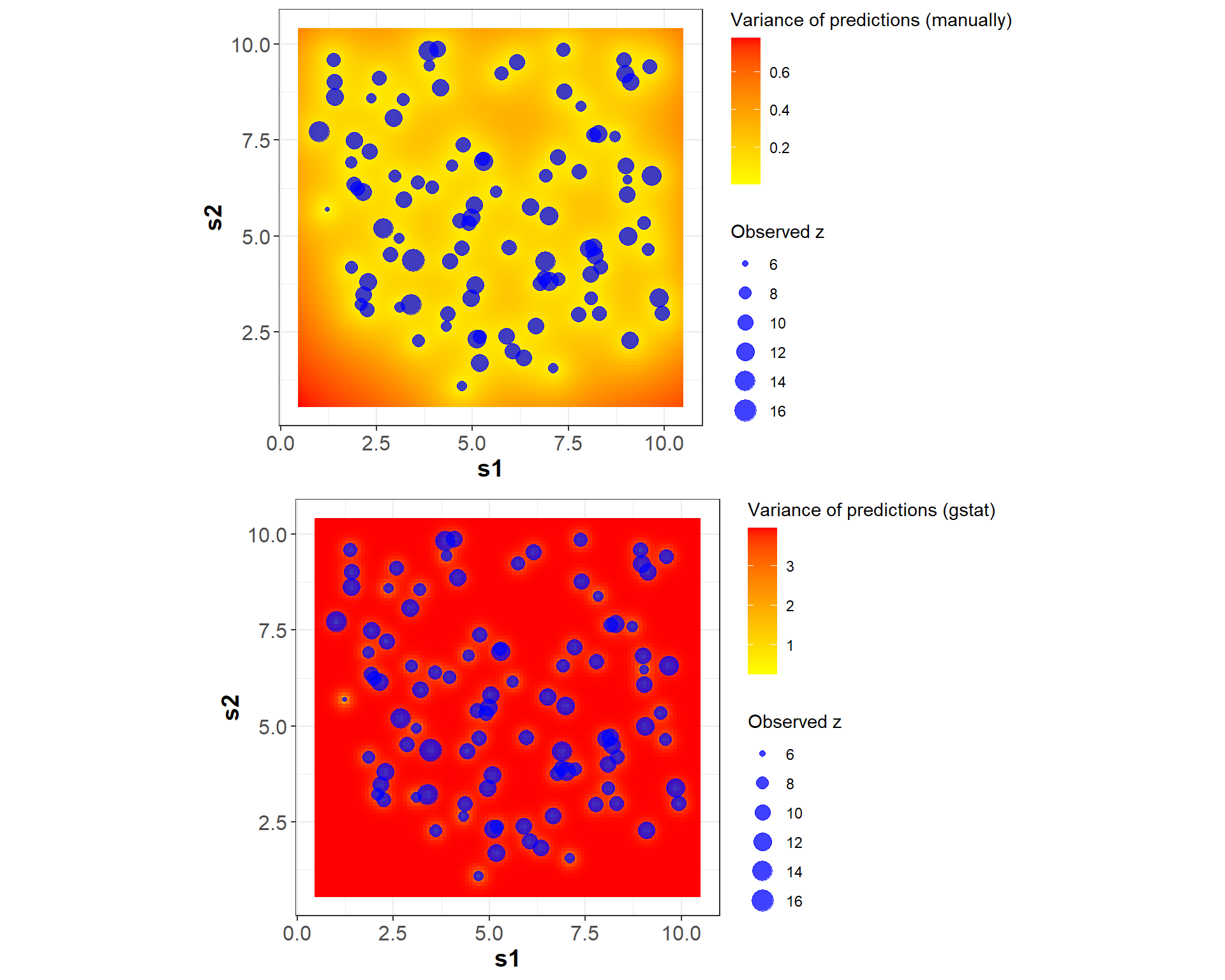
Comparing the prediction in location \(\mathbf{s}_0\), for Kriging computed manually and using “gstat” package, the values are very close (9.516983 and 9.715304, respectively). The variance for the prediction using “gstat” is 3.880513.
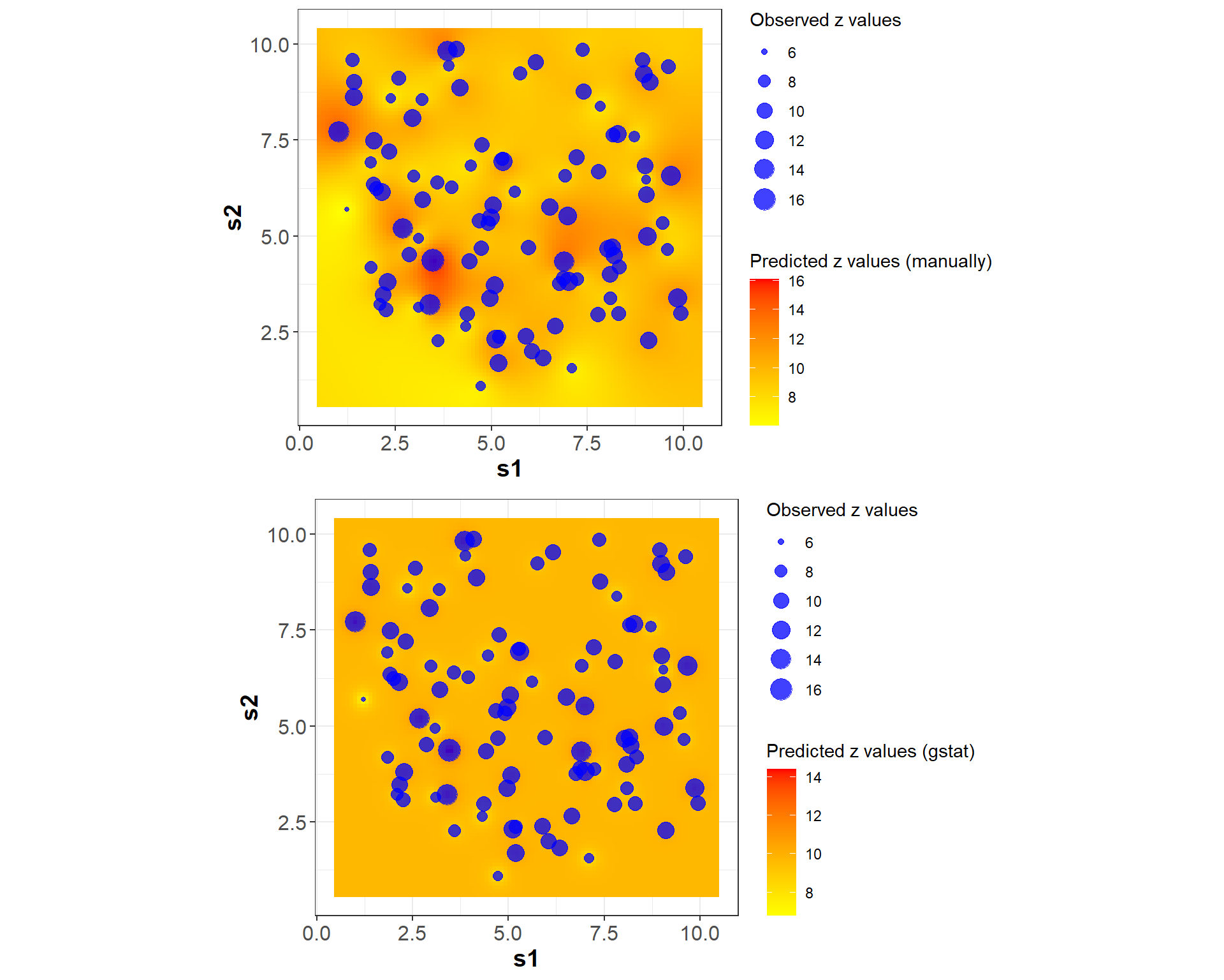
Finally, we can compare the interpolation in a grid for both methods.
#============================================# Interpolation#============================================# Set up prediction gridbbox_vals <-bbox(spat_data)# Extract rangesgrid_size <-100s1_seq <-seq(bbox_vals[1, 1] -0.5, bbox_vals[1, 2] +0.5, length.out = grid_size)s2_seq <-seq(bbox_vals[2, 1] -0.5, bbox_vals[2, 2] +0.5, length.out = grid_size)# Create prediction gridgrid_points <-expand.grid(x = s1_seq, y = s2_seq)# Initialize vector for predictions (interpolation)z_inter <-numeric(nrow(grid_points))var_inter <-numeric(nrow(grid_points))# Loop over grid pointsfor (k in1:nrow(grid_points)) { s0 <-as.numeric(grid_points[k, ])# Build RHS covariance vector c_rhs <-numeric(n +1)for (i in1:n) { h <-sqrt(sum((locations[i, ] - s0)^2)) c_rhs[i] <-exp_cov(h) } c_rhs[n +1] <-1# Solve for weights sol <-solve(cov_mat, c_rhs) w <- sol[1:n]# Kriging estimate z_inter[k] <-sum(w * z_values) var_inter[k] <-exp_cov(0) -sum(w * c_rhs[1:n]) + M}# Reshape result into matrix for plottingz_pred <-matrix(z_inter, nrow = grid_size, ncol = grid_size, byrow =FALSE)z_var <-matrix(var_inter, nrow = grid_size, ncol = grid_size, byrow =FALSE)#====================================# Using the "gstat" package#====================================# Convert grid to SpatialPointscoordinates(grid_points) <-~x + ygridded(grid_points) <-TRUE# Create gstat object for Krigingkrige_gstat <-krige(z_values ~1, spat_data, grid_points, model = fit_vario)
[using ordinary kriging]
z_pred_df <-expand.grid(x = s1_seq, y = s2_seq)# Adding a column of z valuesz_pred_df$z_values <- z_values# Predictionsz_pred_df$z_pred <-as.vector(z_pred) z_pred_df$z_pred_gstat <-as.vector(krige_gstat$var1.pred)# Variancesz_pred_df$z_var <-as.vector(z_var)z_pred_df$z_var_gstat <-as.vector(krige_gstat$var1.var)# Plot prediction + observed pointsspat_data <-data.frame(spat_data)head(spat_data)
In this first entry, I explored the foundational idea of Kriging interpolation, initially proposed by Danie G. Krige and later formalized mathematically by Georges Matheron. The prediction at a specific location, or interpolation over a spatial domain, can be done by solving a system of linear equations. The goal here is to demonstrate that Kriging can be applied both through its classical formulation.
In next post (Understanding Kriging Part 2), I will be presenting its full probabilistic interpretation given by a “Gaussian Process Regression”. While in this post, Kriging predictions or interpolations are based on solving a linear system of equations, a hold understanding of stochastic (spatial) processes is still essential (I did not cover that part given the core of the post, but you can review it in Cressie (1993)). However, the solution itself of the Kriging system of equations relies on linear algebra rather than a likelihood-based method.
Note 1: I am not an expert in using the “gstat"package, so the comparisons presented may not be optimal or the most efficient. The package was used solely for illustrative purposes.
Note 2: It is interesting to see high values for the variance in the interpolation using the “gstat"package. Let’s explore it in the next post..
References
Cressie, Noel AC. 1993. “Spatial Prediction and Kriging.”Statistics for Spatial Data (Cressie NAC, Ed). New York: John Wiley & Sons, 105–209.
Krige, D. G. 1951. “A Statistical Approach to Some Basic Mine Valuation Problems on the Witwatersrand.”Journal of the Chemical, Metallurgical and Mining Society of South Africa 52 (6): 119–39.