library(pacman)
pacman::p_load(tidyverse, dplyr, parallel, ggplot2, mgcv, rstan, gridExtra, bayesplot)1 Overview
This tutorial explains and implements regTPS (link to the paper), a way of approximating a Gaussian random field (GRF) for Bayesian spatial models. The idea is to build the covariance of the field from a regularized thin plate spline (TPS) operator, expand it with a Karhunen-Loève expansion (KLE), and fit the resulting low-dimensional model by MCMC.
Let consider the following spatial model
\[y_i = u(\mathbf{s}_i) + \varepsilon_i, \qquad \varepsilon_i \overset{\text{iid}}{\sim} \mathcal{N}(0, \sigma_\varepsilon^2), \qquad i = 1, \dots, N,\]
where \(\mathbf{s}_i \in \mathcal{D} \subset \mathbb{R}^2\) is a vector of spatial coordinates \(\mathbf{s} = (s_1, s_2)\) and \(u(\cdot)\) is a GRF. In this example, no separate mean is included: the constant function belongs to the polynomial null space of the TPS penalty and is handled by the field itself.
The main steps to follow are:
- Build a TPS basis and its penalty matrix \(\mathbf{S}\) (with
mgcv). - Eigendecompose \(\mathbf{S}\) and order the eigenvalues \(v_k\) in ascending order.
- Truncate the expansion at \(M\) modes using a variance-retention rule.
- Place the prior \(z_k \sim \mathcal{N}\big(0, (1+\alpha v_k)^{-1}\big)\) on the coefficients, written in non-centered form.
- Sample \((\tilde{\mathbf{z}}, \alpha, \sigma_\varepsilon)\) with Stan.
The sections below give the theory, the code and a simulation study.
2 Theory
2.1 Gaussian random field and the Karhunen-Loève expansion
A GRF \(u(\mathbf{s})\) is a collection of random variables such that every finite subset is multivariate normal. It is fully specified by its mean and its covariance function \(C(\mathbf{s}, \mathbf{s}')\). Covariance functions are symmetric and positive semidefinite, and under mild conditions they are Hilbert-Schmidt kernels. Mercer’s theorem then gives
\[C(\mathbf{s}, \mathbf{s}') = \sum_{k=1}^{\infty} \lambda_k \, \phi_k(\mathbf{s})\, \phi_k(\mathbf{s}'),\]
where \((\lambda_k, \phi_k)\) solve the Fredholm eigenproblem
\[\int_{\mathcal{D}} C(\mathbf{s}, \mathbf{s}')\, \phi_k(\mathbf{s}')\, d\mathbf{s}' = \lambda_k \phi_k(\mathbf{s}), \qquad \langle \phi_k, \phi_\ell \rangle_{L^2} = \delta_{k\ell}.\]
Truncating at \(M\) terms gives the KLE of the field,
\[u(\mathbf{s}) \approx \sum_{k=1}^{M} \sqrt{\lambda_k}\, \phi_k(\mathbf{s})\, \epsilon_k, \qquad \epsilon_k \overset{\text{iid}}{\sim} \mathcal{N}(0,1).\]
The practical difficulty is that the eigenpairs are known in closed form only for a few covariances. The regTPS construction avoids this by obtaining the eigensystem from a penalty matrix that is already available in standard spline R package (mgcv).
2.2 Thin plate splines and the bending energy
For \(f \in H^2(\mathcal{D})\) the thin plate spline bending energy is
\[J(f) = \int_{\mathcal{D}} \left[ \left(\frac{\partial^2 f}{\partial s_1^2}\right)^2 + 2\left(\frac{\partial^2 f}{\partial s_1 \partial s_2}\right)^2 + \left(\frac{\partial^2 f}{\partial s_2^2}\right)^2 \right] d\mathbf{s}.\]
Up to boundary terms this equals \(\int_{\mathcal{D}} (\Delta f)^2\, d\mathbf{s}\), and its Euler-Lagrange operator is the biharmonic operator \(\Delta^2\). \(J\) is a seminorm: \(J(f) = 0\) exactly when \(f\) is a polynomial of total degree at most 1, i.e. \(f \in \mathcal{P}_1 = \text{span}\{1, s_1, s_2\}\). This null space has dimension
\[d_{\text{null}} = \binom{d + m - 1}{d} = 3 \qquad (d = 2,\ m = 2).\]
A smoothing TPS minimizes the penalized least squares functional
\[\mathcal{L}(f) = \sum_{i=1}^{N} \big(y_i - f(\mathbf{s}_i)\big)^2 + \alpha\, J(f), \qquad \alpha > 0.\]
The TPS kernel \(\phi(\mathbf{d}) = \mathbf{d}^2 \log \mathbf{d}\), with \(\mathbf{d} = ||\mathbf{s} - \mathbf{s'}||\) is the Euclidean distance, is the Green’s function of \(\Delta^2\) in \(\mathbb{R}^2\) (up to the constant \(1/8\pi\)). It is only conditionally positive definite, so it is not a valid covariance function, and Mercer’s theorem and the KLE cannot be applied to it directly.
2.3 Regularizing the operator
To obtain a proper covariance, regTPS replaces the singular biharmonic operator by the regularized elliptic operator
\[L_\alpha = \mathbf{I} + \alpha \Delta^2, \qquad \alpha > 0.\]
It arises from the continuous variational problem
\[\min_{f \in H^2(\mathcal{D})} \int_{\mathcal{D}} (f - g)^2\, d\mathbf{s} + \alpha J(f),\]
whose Euler-Lagrange equation is the fourth-order elliptic PDE \(L_\alpha f = g\). Under suitable boundary conditions \(L_\alpha\) is self-adjoint and boundedly invertible, and its inverse
\[(L_\alpha^{-1} g)(\mathbf{s}) = \int_{\mathcal{D}} K_\alpha(\mathbf{s}, \mathbf{s}')\, g(\mathbf{s}')\, d\mathbf{s}'\]
is compact, self-adjoint and strictly positive definite. Its kernel \(K_\alpha\) is therefore a Hilbert-Schmidt kernel, and Mercer’s theorem applies:
\[K_\alpha(\mathbf{s}, \mathbf{s}') = \sum_{k=1}^{\infty} \lambda_{k,\alpha}\, \phi_k(\mathbf{s})\, \phi_k(\mathbf{s}').\]
2.3.1 The spectrum of \(L_\alpha\)
Let \(v_k\) denote the eigenvalues of \(\Delta^2\) in ascending order, so \(\Delta^2 \phi_k = v_k \phi_k\). Because \(L_\alpha\) is a polynomial in \(\Delta^2\), it shares the eigenfunctions \(\phi_k\), and
\[L_\alpha \phi_k = (1 + \alpha v_k)\, \phi_k \quad\Longrightarrow\quad \mu_k(\alpha) = 1 + \alpha v_k, \qquad \boxed{\;\lambda_{k,\alpha} = \frac{1}{1 + \alpha v_k}\;}\]
The spectrum has two regimes:
| Modes | Eigenvalue of \(\Delta^2\) | KLE variance \(\lambda_{k,\alpha}\) | Interpretation |
|---|---|---|---|
| \(k \le d_{\text{null}}\) | \(v_k = 0\) | \(1\) | Polynomial trends, unpenalized, unit prior variance |
| \(k > d_{\text{null}}\) | \(v_k > 0\), increasing | \((1+\alpha v_k)^{-1} < 1\), decreasing | Increasingly oscillatory modes, shrunk more strongly |
The parameter \(\alpha\) controls how fast \(\lambda_{k,\alpha}\) decays: larger \(\alpha\) shrinks rough modes harder and gives smoother, longer-range fields. It does not change the smoothness class of the field. The order of the operator does, and for \(\Delta^2\) in two dimensions the Matérn-type smoothness is \(\nu = \ell - d/2 = 2 - 1 = 1\).
Treating the null space explicitly, with unit variance, is a central feature of the method. The polynomial part is neither projected out nor penalized, so the field can represent large-scale trends.
2.4 Finite-dimensional (Ritz-Galerkin) approximation
The eigenfunctions \(\phi_k\) are not available in closed form on a general domain. They are approximated in the space spanned by \(K\) TPS basis functions,
\[\mathcal{V}_K = \text{span}\{\tilde\phi_1, \dots, \tilde\phi_K\}, \qquad \tilde{\boldsymbol\phi}(\mathbf{s}) = \big(\tilde\phi_1(\mathbf{s}), \dots, \tilde\phi_K(\mathbf{s})\big)^\top,\]
which in practice is the thin plate regression spline basis of mgcv (bs = "tp", k = K). In this basis, \(f(\mathbf{s}) = \tilde{\boldsymbol\phi}(\mathbf{s})^\top \mathbf{c}\) and the bending energy becomes a quadratic form,
\[J(f) = \mathbf{c}^\top \mathbf{S}\, \mathbf{c}, \qquad S_{jl} = \int_{\mathcal{D}} \Delta\tilde\phi_j(\mathbf{s})\, \Delta\tilde\phi_l(\mathbf{s})\, d\mathbf{s}.\]
The matrix \(\mathbf{S}\) is symmetric positive semidefinite, with a null space of dimension \(d_{\text{null}}\). mgcv computes it in a numerically stable way without evaluating the integral. It is essential to build the basis without the sum-to-zero constraint (absorb.cons = FALSE), so that the constant and linear terms stay in the basis.
2.4.1 Eigendecomposition of the penalty
\[\mathbf{S} = \boldsymbol\Psi_S\, \mathbf{V}_S\, \boldsymbol\Psi_S^\top, \qquad \mathbf{V}_S = \text{diag}(v_1 \le v_2 \le \dots \le v_K), \qquad \boldsymbol\Psi_S^\top \boldsymbol\Psi_S = \mathbf{I}_K.\]
The first \(d_{\text{null}}\) eigenvalues are numerically zero and their eigenvectors span the polynomial trends. The \(k\)-th discrete eigenfunction is
\[\hat\phi_k(\mathbf{s}) = \tilde{\boldsymbol\phi}(\mathbf{s})^\top \boldsymbol\psi_{S,k}.\]
The eigenvalues \(v_k\) of \(\mathbf{S}\) approximate those of \(\Delta^2\) on \(\mathcal{V}_K\), and the approximation improves as \(K\) grows.
Standard versus generalized eigenproblem. A fully consistent Galerkin discretization solves the generalized problem \(\mathbf{S}\boldsymbol\psi = v\,\mathbf{M}\boldsymbol\psi\) with the \(L^2\) mass matrix \(M_{jk} = \int \tilde\phi_j\tilde\phi_k\, d\mathbf{s}\), which keeps the \(\hat\phi_k\) orthonormal in \(L^2\). regTPS instead solves the standard problem \(\mathbf{S}\boldsymbol\psi = v\boldsymbol\psi\), as is common in TPS software. Modes are then ranked purely by bending energy, and \(\alpha\) absorbs any constant scaling. This is a computational approximation (see Appendix A of the paper).
2.5 Discrete KLE with adaptive truncation
With the discrete eigenpairs, the covariance kernel is approximated by
\[K_\alpha(\mathbf{s}, \mathbf{s}') \approx \sum_{k=1}^{M} \lambda_{k,\alpha}\, \hat\phi_k(\mathbf{s})\, \hat\phi_k(\mathbf{s}'), \qquad \lambda_{k,\alpha} = \frac{1}{1 + \alpha v_k}.\]
The truncation level \(M \le K\) is chosen to retain a proportion \(\gamma\) (typically 0.95 to 0.99) of the total KLE variance:
\[M = \min\left\{ m : \frac{\sum_{k=1}^{m} \lambda_{k,\alpha}}{\sum_{k=1}^{K} \lambda_{k,\alpha}} \ge \gamma \right\}.\]
Because the truncation is decided before sampling, it needs a fixed reference value of \(\alpha\). The implementation below uses
\[\alpha_{\text{ref,scaled}} = \frac{\alpha_{\text{ref}}}{\text{median}\{v_k : v_k > 10^{-10}\}},\]
which makes the truncation rule independent of the numerical scale of \(\mathbf{S}\). It also forces \(\lambda_k = 1\) for \(k \le d_{\text{null}}\) and requires \(M \ge d_{\text{null}} + 5\), so that a few penalized modes are always kept. This \(\alpha_{\text{ref,scaled}}\) is used only to choose \(M\) and to initialize the sampler. The \(\alpha\) that enters the prior is estimated.
2.6 Bayesian formulation
2.6.1 Prior on the coefficients
Writing \(f = \tilde{\boldsymbol\phi}^\top\mathbf{c}\), the penalty \(J(f) = \mathbf{c}^\top\mathbf{S}\mathbf{c}\) corresponds to a Gaussian prior on \(\mathbf{c}\) with precision matrix
\[\mathbf{P}_\alpha = \mathbf{I} + \alpha\mathbf{S}, \qquad \mathbf{c} \sim \mathcal{N}\big(\mathbf{0}, \mathbf{P}_\alpha^{-1}\big).\]
In the rotated coordinates \(\mathbf{z} = \boldsymbol\Psi_S^\top \mathbf{c}\), the precision becomes diagonal, \(\mathbf{I} + \alpha\mathbf{V}_S\), so the components are independent:
\[z_k \sim \mathcal{N}\left(0, \lambda_{k,\alpha}\right), \qquad \lambda_{k,\alpha} = \frac{1}{1 + \alpha v_k}.\]
The field is then \(f(\mathbf{s}) = \sum_{k=1}^{M} z_k \hat\phi_k(\mathbf{s}) = \boldsymbol\Phi(\mathbf{s})^\top\mathbf{z}\).
2.6.2 Non-centered parameterization
To decouple the latent coefficients from the hyperparameter \(\alpha\) and improve HMC geometry, we sample standard normal variables \(\tilde z_k\) and set
\[z_k = \sqrt{\lambda_{k,\alpha}}\,\tilde z_k = \begin{cases} \tilde z_k, & k \le d_{\text{null}},\\[4pt] \dfrac{\tilde z_k}{\sqrt{1 + \alpha v_k}}, & k > d_{\text{null}}, \end{cases} \qquad \tilde z_k \overset{\text{iid}}{\sim} \mathcal{N}(0,1).\]
2.6.3 Likelihood and priors
Let \(\boldsymbol\Psi_M \in \mathbb{R}^{K\times M}\) contain the first \(M\) eigenvectors and \(\tilde{\boldsymbol\Phi} \in \mathbb{R}^{N\times K}\) the TPS basis at the observed sites. The KLE design matrices are
\[\boldsymbol\Phi_{\text{obs}} = \tilde{\boldsymbol\Phi}\,\boldsymbol\Psi_M \in \mathbb{R}^{N\times M}, \qquad \boldsymbol\Phi_{\text{grid}} = \tilde{\boldsymbol\Phi}_{\text{grid}}\,\boldsymbol\Psi_M,\]
and the likelihood is
\[\mathbf{y} \mid \tilde{\mathbf{z}}, \alpha, \sigma_\varepsilon \sim \mathcal{N}\big(\boldsymbol\Phi_{\text{obs}}\,\mathbf{z}(\tilde{\mathbf{z}}, \alpha),\ \sigma_\varepsilon^2 \mathbf{I}_N\big).\]
The hyperpriors are
\[\begin{aligned} \sigma_\varepsilon &\sim \text{Exponential}(\lambda_\sigma), \qquad \lambda_\sigma = -\frac{\log p_\sigma}{\sigma_0}, \quad \Pr(\sigma_\varepsilon > \sigma_0) = p_\sigma,\\ \log\alpha &\sim \mathcal{N}(0, \sigma_\alpha^2),\\ \tilde z_k &\sim \mathcal{N}(0, 1), \qquad k = 1,\dots,M. \end{aligned}\]
The exponential prior on \(\sigma_\varepsilon\) is a penalized complexity (PC) prior. We use \(\sigma_0 = 0.5\) and \(p_\sigma = 0.05\). The joint posterior is
\[p(\tilde{\mathbf{z}}, \alpha, \sigma_\varepsilon \mid \mathbf{y}) \propto \left[\prod_{i=1}^{N} \mathcal{N}\big(y_i \mid (\boldsymbol\Phi_{\text{obs}}\mathbf{z})_i, \sigma_\varepsilon^2\big)\right] \prod_{k=1}^{M}\mathcal{N}(\tilde z_k \mid 0, 1)\ \pi(\alpha)\ \pi(\sigma_\varepsilon).\]
2.6.4 Prediction
For any set of new locations, the field is \(\boldsymbol\Phi_{\text{new}}\mathbf{z}\) with \(\boldsymbol\Phi_{\text{new}} = \tilde{\boldsymbol\Phi}_{\text{new}}\boldsymbol\Psi_M\). Each posterior draw of \(\mathbf{z}\) gives one draw of the field, so uncertainty in \(\alpha\), \(\sigma_\varepsilon\) and the coefficients propagates automatically.
2.7 From the theory to the code
| Quantity | Math | R object | Stan variable |
|---|---|---|---|
| Number of TPS basis functions | \(K\) | k_basis |
|
| Penalty matrix | \(\mathbf{S}\) | sm$S[[1]] |
|
| Penalty eigenvalues (first \(M\)) | \(v_k\) | S_diag_truncated |
S_diag_truncated |
| Retained eigenvectors | \(\boldsymbol\Psi_M\) | evectors[, 1:M] |
|
| KLE design at observed sites | \(\boldsymbol\Phi_{\text{obs}}\) | Phi_kle_sp |
Phi_kle_sp |
| KLE design at prediction grid | \(\boldsymbol\Phi_{\text{grid}}\) | Phi_kle_grid |
Phi_kle_grid |
| Truncation level | \(M\) | M_truncation |
M |
| Null-space dimension | \(d_{\text{null}}\) | M_P_null_space |
M0 |
| Variance threshold | \(\gamma\) | variance_threshold |
|
| Smoothing parameter | \(\alpha\) | alpha = exp(logalpha) |
|
| Whitened coefficients | \(\tilde z_k\) | z_tilde |
|
| Scaled coefficients | \(z_k\) | z |
|
| Noise sd | \(\sigma_\varepsilon\) | sigma |
|
| PC prior rate | \(\lambda_\sigma\) | lambda_sigma_e |
lambda_sigma_e |
3 Implementation in R
First, we will load the main libraries used for this example:
3.1 The regTPS function
regTPS_s() performs steps 1 to 3. It contains no inference code and returns everything needed by the Stan model.
regTPS_s <- function(sp_points, grid_total, y_obs, k_basis,
                     variance_threshold = 0.95, alpha_ref = 1,
                     verbose = TRUE) {

  #====================================
  # Basis and penalty (no centering constraint, so the null space is kept)
  #====================================
  data_smooth <- data.frame(s1 = sp_points$s1, s2 = sp_points$s2, y_obs = y_obs)
  sm <- mgcv::smoothCon(s(s1, s2, k = k_basis, bs = "tp"),
                        data = data_smooth, absorb.cons = FALSE)[[1]]

  Phi_basis_sp   <- PredictMat(sm, data_smooth)
  Phi_basis_grid <- PredictMat(sm, grid_total)
  S <- sm$S[[1]]

  #====================================
  # Eigendecomposition (S psi = v psi), cleaned and ordered ascending
  #====================================
  S_eig    <- eigen(S, symmetric = TRUE)
  S_diag   <- S_eig$values
  evectors <- S_eig$vectors

  S_diag[abs(S_diag) < 1e-12] <- 0
  if (any(S_diag < -1e-10))
    warning("Negative eigenvalues detected (max magnitude: ",
            max(abs(S_diag[S_diag < 0])), ")")
  S_diag[S_diag < 0] <- 0

  order_idx <- order(S_diag, decreasing = FALSE)
  S_diag    <- S_diag[order_idx]
  evectors  <- evectors[, order_idx]

  M_P_null_space <- sm$null.space.dim

  #====================================
  # Variance-based truncation
  #====================================
  nonzero_eigs <- S_diag[S_diag > 1e-10]
  if (length(nonzero_eigs) == 0) stop("No non-zero eigenvalues found.")

  # reference alpha, rescaled so that the rule does not depend on the scale of S
  alpha_ref_scaled <- alpha_ref / median(nonzero_eigs)
  lambda_k <- 1 / (1 + alpha_ref_scaled * S_diag)
  lambda_k[1:M_P_null_space] <- 1            # null space: unit variance

  total_variance <- sum(lambda_k)
  cumvar <- cumsum(lambda_k) / total_variance

  M_truncation <- which(cumvar >= variance_threshold)[1]
  if (is.na(M_truncation)) M_truncation <- length(S_diag)

  M_truncation <- max(M_truncation, M_P_null_space + 5)
  if (M_truncation < M_P_null_space) M_truncation <- M_P_null_space

  var_explained <- sum(lambda_k[1:M_truncation]) / total_variance

  if (verbose) {
    cat("Null space dim:", M_P_null_space, "| basis:", length(S_diag),
        "| non-zero eig:", sum(S_diag > 1e-10), "\n")
    cat("alpha_ref scaled:", round(alpha_ref_scaled, 6),
        "| M_truncation:", M_truncation,
        "| variance explained:", round(100 * var_explained, 2), "%\n")
  }

  #====================================
  # Truncated matrices
  #====================================
  idx <- 1:M_truncation
  Phi_kle_sp       <- Phi_basis_sp   %*% evectors[, idx]
  Phi_kle_grid     <- Phi_basis_grid %*% evectors[, idx]
  S_diag_truncated <- S_diag[idx]

  list(Phi_kle_sp         = Phi_kle_sp,
       Phi_kle_grid       = Phi_kle_grid,
       S_diag_truncated   = S_diag_truncated,
       M_truncation       = M_truncation,
       M_P_null_space     = M_P_null_space,
       alpha_ref_scaled   = alpha_ref_scaled,
       variance_explained = var_explained,
       k_basis            = k_basis,
       S_diag_full        = S_diag,
       lambda_k           = lambda_k,
       cumvar             = cumvar,
       evectors           = evectors,
       sm                 = sm)
}
The objects nedded to use regTPS_s() are:
sp_points,grid_total: data frames with columnss1ands2, for the observed sites and the prediction locations. The column names must be exactly these because they appear in themgcvformula.y_obs: the response variable, used only to build the smoothing data frame.k_basis: the number of TPS basis functions \(K\). It must be smaller than the number of distinct sites.variance_threshold: the proportion \(\gamma\) of KLE variance to retain.alpha_ref: the reference \(\alpha\) used for the truncation rule.
4 Stan model
The Stan program is a direct transcription of the non-centered model above. The mian code is the following:
// regTPS spatial model (non-centered parameterization)

data {
  int<lower=1> N;                 // number of observations
  int<lower=1> N_grid;            // number of prediction grid points
  int<lower=1> M;                 // M_truncation
  int<lower=0, upper=M> M0;       // null-space dimension
  vector[N] y_obs;
  matrix[N, M] Phi_kle_sp;        // KLE design at observed sites
  matrix[N_grid, M] Phi_kle_grid; // KLE design at prediction grid
  vector[M] S_diag_truncated;     // penalty eigenvalues v_k
  real<lower=0> lambda_sigma_e;   // exponential (PC) prior rate for sigma_e
  real<lower=0> sigma_logalpha;   // prior sd of log(alpha)
}

parameters {
  vector[M] z_tilde;              // whitened coefficients
  real logalpha;
  real<lower=0> sigma_e;          // Stan adds the log-Jacobian automatically
}

transformed parameters {
  real alpha = exp(logalpha);
  vector[M] scale;                // sqrt(lambda_k)
  vector[M] z;
  vector[N] field_sp;

  for (k in 1:M) {
    if (k <= M0) {
      scale[k] = 1.0;             // null space unpenalized
    } else {
      scale[k] = 1.0 / sqrt(1.0 + alpha * S_diag_truncated[k] + 1e-10);
    }
  }
  z = scale .* z_tilde;
  field_sp = Phi_kle_sp * z;
}

model {
  // priors
  sigma_e  ~ exponential(lambda_sigma_e);
  logalpha ~ normal(0, sigma_logalpha);
  z_tilde  ~ std_normal();

  // likelihood
  y_obs ~ normal(field_sp, sigma_e);
}

generated quantities {
  vector[N_grid] field_grid = Phi_kle_grid * z;
  vector[N] y_sim;
  vector[N] log_lik;

  for (i in 1:N) {
    y_sim[i]   = normal_rng(field_sp[i], sigma_e);
    log_lik[i] = normal_lpdf(y_obs[i] | field_sp[i], sigma_e);
  }
}
Points worth noting:
- Null space. The
if (k <= M0)branch gives the polynomial modes unit scale, so they carry a \(\mathcal{N}(0,1)\) prior and no smoothing. - Hyperparameters. There are only two, \(\alpha\) and \(\sigma_\varepsilon\). No range or marginal variance of a covariance function is estimated.
- Jacobian. Declaring
sigmawith<lower=0>makes Stan sample on the log scale and add the Jacobian itself. This is what thenlp -= logsigmaline did in the TMB version. - Generated quantities.
field_gridis the posterior field on the prediction grid,y_simsupports posterior predictive checks, andlog_liksupports LOO cross-validation.
5 Simulation study
5.1 Simulate a Matérn field with Gaussian noise
We simulate a Matérn (\(\nu = 3/2\)) field jointly at 200 random observed sites and a \(30\times 30\) prediction grid, then add Gaussian noise at the observed sites. The fitted model uses a TPS prior, so it is not the true data-generating covariance; this is the usual stress test for the approximation.
set.seed(123)

# Settings
n_obs       <- 200     # number of observed locations
n_grid_pred <- 30      # prediction grid is n_grid_pred x n_grid_pred
sigma_e     <- 0.5     # true noise sd
sigma_u     <- 1.0     # true marginal sd of the field
range_u     <- 0.3     # spatial range (domain is [0,1]^2)
mu0         <- 0       # constant mean

# Locations
sp_points  <- data.frame(s1 = runif(n_obs), s2 = runif(n_obs))
g          <- seq(0, 1, length.out = n_grid_pred)
grid_total <- expand.grid(s1 = g, s2 = g)

all_pts <- rbind(sp_points, grid_total)
n_sp    <- nrow(sp_points)
n_grid  <- nrow(grid_total)

# True covariance (Matern, nu = 3/2)
matern32 <- function(d, sigma, rho) {
  h <- sqrt(3) * d / rho
  sigma^2 * (1 + h) * exp(-h)
}
D        <- as.matrix(dist(all_pts))
Cov_true <- matern32(D, sigma_u, range_u)

# Simulate the field at observed and grid locations jointly
L     <- chol(Cov_true + diag(1e-8, nrow(Cov_true)))   # upper triangular
u_all <- mu0 + as.vector(t(L) %*% rnorm(nrow(Cov_true)))

u_true_sp   <- u_all[1:n_sp]
u_true_grid <- u_all[(n_sp + 1):(n_sp + n_grid)]

# Gaussian observation noise
y_obs <- u_true_sp + rnorm(n_sp, mean = 0, sd = sigma_e)image(g, g, matrix(u_true_grid, n_grid_pred, n_grid_pred),
xlab = "s1", ylab = "s2", main = "True field")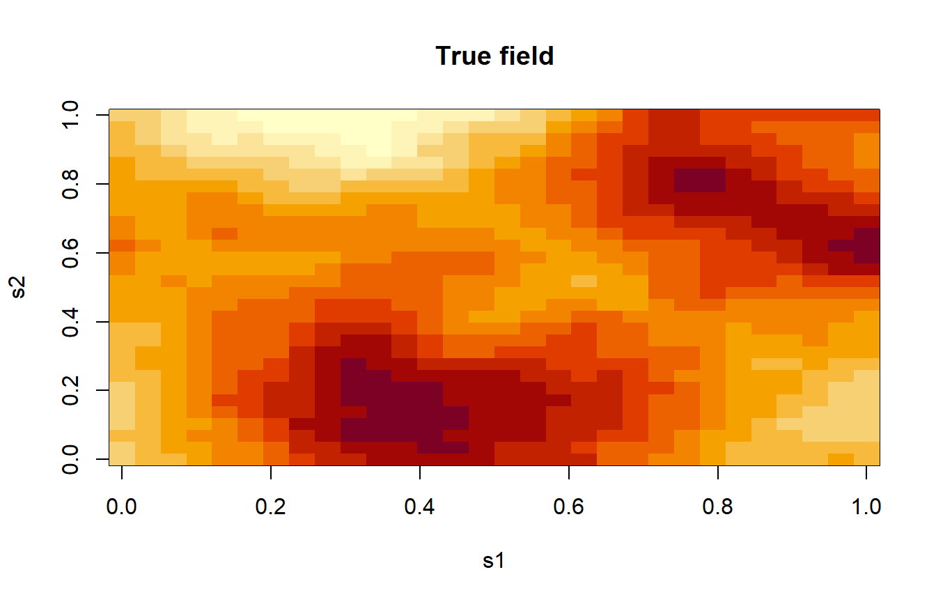
5.2 Build the regTPS basis
We use \(K = 199\) basis functions (one fewer than the number of observed sites, to avoid singularities) and keep 95% of the KLE variance.
K <- 199
variance_threshold <- 0.95

reg <- regTPS_s(sp_points, grid_total, y_obs, k_basis = K,
                variance_threshold = variance_threshold, alpha_ref = 1)
Null space dim: 3 | basis: 199 | non-zero eig: 196
alpha_ref scaled: 0.020242 | M_truncation: 151 | variance explained: 95.04 %5.2.1 Inspecting the spectrum and the truncation
The penalty eigenvalues are zero for the first \(d_{\text{null}} = 3\) modes and then grow quickly. The KLE variances \(\lambda_k\) therefore decay, and the cumulative variance saturates well before \(K\) modes.
M  <- reg$M_truncation
M0 <- reg$M_P_null_space
K  <- length(reg$S_diag_full)

df_spec <- data.frame(k = 1:K, v = reg$S_diag_full,
                      type = ifelse(1:K <= M0, "Null space", "Penalized"))

p_spec <- ggplot(df_spec, aes(k, pmax(v, 1e-6), colour = type)) +
  geom_point(size = 1.2) +
  geom_vline(xintercept = M, linetype = 2) +
  scale_y_log10() +
  labs(title = "Penalty eigenvalues", x = "Mode index (increasing roughness)",
       y = expression(v[k]~"(null modes floored at 1e-6)"), colour = NULL) +
  theme_bw()

df_cum <- data.frame(k = 1:K, cumvar = reg$cumvar)

p_cum <- ggplot(df_cum, aes(k, cumvar)) +
  geom_line() +
  geom_hline(yintercept = variance_threshold, linetype = 2) +
  geom_vline(xintercept = M, linetype = 2) +
  labs(title = paste0("Cumulative variance (M = ", M, ")"),
       x = "Number of basis functions", y = "Cumulative proportion") +
  theme_bw()

grid.arrange(p_spec, p_cum, ncol = 2)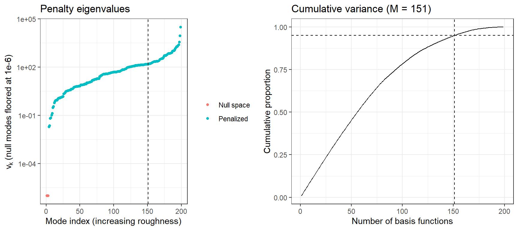
6 Bayesian inference with Stan
6.1 Data, priors and initial values
The PC prior for \(\sigma_\varepsilon\) states \(\Pr(\sigma_\varepsilon > 1) = 0.05\). For \(\log\alpha\) we use \(\mathcal{N}(0, \sigma_\alpha^2)\). The value of \(\sigma_{\alpha}\) is fixed at 1 in this example and passed to Stan as a data input.
no_cores <- max(1, min(4, parallel::detectCores() - 1))
options(mc.cores = no_cores)
rstan_options(auto_write = TRUE)

sigma_prior_s0    <- 1.0     # P(sigma > 1) = 0.05
sigma_prior_alpha <- 0.05
lambda_sigma_e    <- -log(sigma_prior_alpha) / sigma_prior_s0
sigma_logalpha    <- 1.0

stan_dat <- list(N                = length(y_obs),
                 N_grid           = nrow(reg$Phi_kle_grid),
                 M                = reg$M_truncation,
                 M0               = reg$M_P_null_space,
                 y_obs            = as.vector(y_obs),
                 Phi_kle_sp       = unname(as.matrix(reg$Phi_kle_sp)),
                 Phi_kle_grid     = unname(as.matrix(reg$Phi_kle_grid)),
                 S_diag_truncated = as.vector(reg$S_diag_truncated),
                 lambda_sigma_e   = lambda_sigma_e,
                 sigma_logalpha   = sigma_logalpha)

logalpha_init <- max(min(log(reg$alpha_ref_scaled), 3), -3)
sigma_init    <- sd(y_obs)

stan_init <- function(chain_id) {
  list(z_tilde  = as.array(rep(0, reg$M_truncation)),
       logalpha = logalpha_init,
       sigma_e  = sigma_init)
}
6.2 Sampling
The fit is cached in regTPS_fit.rds. If the file exists and matches the current basis, it is read and no sampling is done; otherwise the model is sampled and the file is written. Delete regTPS_fit.rds after changing the data, the priors or the Stan program.
fit_file <- "regTPS_fit.rds"

# read the saved fit if there is one
stan_fit <- if (file.exists(fit_file)) readRDS(fit_file) else NULL

# the saved fit must have the same number of modes as the current basis
fit_ok <- !is.null(stan_fit) &&
  ncol(rstan::extract(stan_fit, pars = "z")$z) == reg$M_truncation

if (!fit_ok) {
  if (!exists("regTPS_mod"))
    stop("No valid saved fit and the Stan model was not compiled. ",
         "Enable the stan-model chunk and render again.")

  stan_fit <- sampling(regTPS_mod,
                       data    = stan_dat,
                       init    = stan_init,
                       chains  = 3, iter = 2000, warmup = 1000, seed = 123,
                       control = list(max_treedepth = 12, adapt_delta = 0.95),
                       cores   = no_cores,
                       refresh = 0)
  saveRDS(stan_fit, fit_file)
}

# Extract the posteriors
post <- rstan::extract(stan_fit)
6.3 Convergence and hyperparameters
print(stan_fit, pars = c("alpha", "sigma_e"), probs = c(0.025, 0.5, 0.975))Inference for Stan model: anon_model.
3 chains, each with iter=2000; warmup=1000; thin=1;
post-warmup draws per chain=1000, total post-warmup draws=3000.
mean se_mean sd 2.5% 50% 97.5% n_eff Rhat
alpha 69.40 0.9 20.64 37.22 66.84 116.36 530 1.01
sigma_e 0.49 0.0 0.03 0.43 0.49 0.55 2140 1.00
Samples were drawn using NUTS(diag_e) at Wed Nov 18 09:38:35 2026.
For each parameter, n_eff is a crude measure of effective sample size,
and Rhat is the potential scale reduction factor on split chains (at
convergence, Rhat=1).rstan::check_hmc_diagnostics(stan_fit)
Divergences:
Tree depth:
Energy:rstan::traceplot(stan_fit, pars = c("alpha", "sigma_e"), ncol = 2)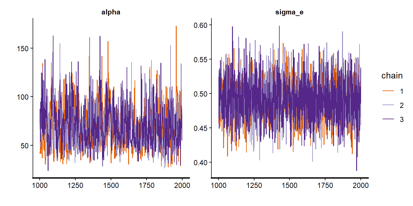
The true noise standard deviation is 0.5. The posterior of \(\log\alpha\) can be compared with its prior to see how much the data inform the smoothing:
ggplot(data.frame(logalpha = post$logalpha), aes(logalpha)) +
  geom_density(fill = "steelblue", alpha = 0.4) +
  stat_function(fun = dnorm, args = list(mean = 0, sd = sigma_logalpha),
                colour = "red") +
  labs(title = expression("Posterior (blue) and prior (red) of"~log~alpha),
       x = expression(log~alpha), y = "Density") +
  theme_bw()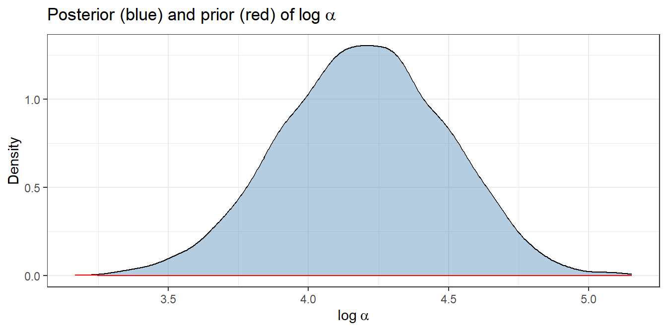
6.4 How the prior and the data interact mode by mode
For each retained mode we compare the posterior mean of \(|z_k|\) with the prior standard deviation \(\sqrt{\lambda_{k,\alpha}}\) (averaged over the posterior of \(\alpha\)). Under a prior-dominated mode, \(\mathbb{E}|z_k| = \sqrt{2/\pi}\,\text{SD}_{\text{prior}}(z_k)\), which is the dashed line. Points above the line indicate that the data push the coefficient to larger values than the prior alone would; points near or below it indicate little data-driven learning. The null-space modes (unit prior SD) separate clearly from the penalized ones.
M  <- reg$M_truncation
M0 <- reg$M_P_null_space

df_z <- data.frame(prior_sd = colMeans(post$scale),
                   abs_z    = abs(colMeans(post$z)),
                   type     = ifelse(1:M <= M0, "Null space", "Penalized"))

ggplot(df_z, aes(prior_sd, abs_z, colour = type, shape = type)) +
  geom_point(size = 2) +
  geom_abline(slope = 1, intercept = log10(sqrt(2 / pi)), linetype = 2) +
  scale_x_log10() + scale_y_log10() +
  labs(x = expression("Prior SD"~sqrt(lambda[k])),
       y = expression("|Posterior mean of"~z[k]~"|"),
       colour = NULL, shape = NULL) +
  theme_bw()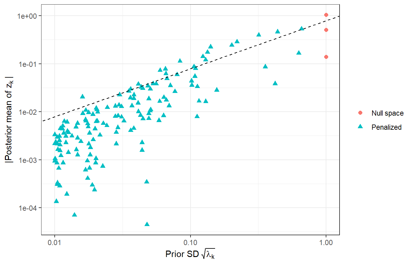
7 Results: true versus estimated field
7.1 Posterior summaries on the grid
spat_field <- post$field_grid        # draws x N_grid

post_mean <- colMeans(spat_field)
post_sd   <- apply(spat_field, 2, sd)
post_lo   <- apply(spat_field, 2, quantile, 0.025)
post_hi   <- apply(spat_field, 2, quantile, 0.975)

df <- data.frame(s1 = grid_total$s1, s2 = grid_total$s2,
                 truth = u_true_grid, post_mean = post_mean, post_sd = post_sd,
                 err = post_mean - u_true_grid,
                 inside = u_true_grid >= post_lo & u_true_grid <= post_hi)

rmse     <- sqrt(mean(df$err^2))
mae      <- mean(abs(df$err))
r2       <- 1 - sum(df$err^2) / sum((df$truth - mean(df$truth))^2)
corr     <- cor(df$truth, df$post_mean)
coverage <- mean(df$inside)

data.frame(RMSE = rmse, MAE = mae, R2 = r2, Correlation = corr,
           Coverage95 = coverage)
RMSE MAE R2 Correlation Coverage95
1 0.2567231 0.2020202 0.9115277 0.9561553 0.9433333Here \(R^2 = 1 - \sum_i (\hat u_i - u_i)^2 / \sum_i (u_i - \bar u)^2\) and Coverage95 is the proportion of grid points whose true value lies inside the 95% credible interval.
7.2 Maps
lims       <- range(c(df$truth, df$post_mean))
fld_scale  <- scale_fill_viridis_c(limits = lims, option = "D")
base_theme <- theme_minimal() + theme(panel.grid = element_blank())

p_true <- ggplot(df, aes(s1, s2, fill = truth)) +
  geom_raster() + fld_scale + coord_equal() +
  labs(title = "True GRF", fill = "u") + base_theme

p_est <- ggplot(df, aes(s1, s2, fill = post_mean)) +
  geom_raster() + fld_scale + coord_equal() +
  labs(title = "Posterior mean", fill = "u") + base_theme

p_err <- ggplot(df, aes(s1, s2, fill = err)) +
  geom_raster() + coord_equal() +
  scale_fill_gradient2(low = "blue", mid = "white", high = "red", midpoint = 0) +
  labs(title = "Error (posterior mean - truth)", fill = "err") + base_theme

p_sd <- ggplot(df, aes(s1, s2, fill = post_sd)) +
  geom_raster() + coord_equal() +
  scale_fill_viridis_c(option = "magma") +
  labs(title = "Posterior SD", fill = "sd") + base_theme

p_scatter <- ggplot(df, aes(truth, post_mean)) +
  geom_point(alpha = 0.4, size = 0.8) +
  geom_abline(slope = 1, intercept = 0, colour = "red") +
  labs(title = sprintf("Truth vs estimate (RMSE = %.3f)", rmse),
       x = "True field", y = "Posterior mean") +
  theme_bw()

p_cover <- ggplot(df, aes(s1, s2, fill = inside)) +
  geom_raster() + coord_equal() +
  scale_fill_manual(values = c("TRUE" = "grey85", "FALSE" = "red"),
                    labels = c("TRUE" = "inside", "FALSE" = "outside")) +
  labs(title = sprintf("95%% CI coverage: %.1f%%", 100 * coverage),
       fill = "truth") + base_theme

grid.arrange(p_true, p_est, p_err, p_sd, p_scatter, p_cover, ncol = 3)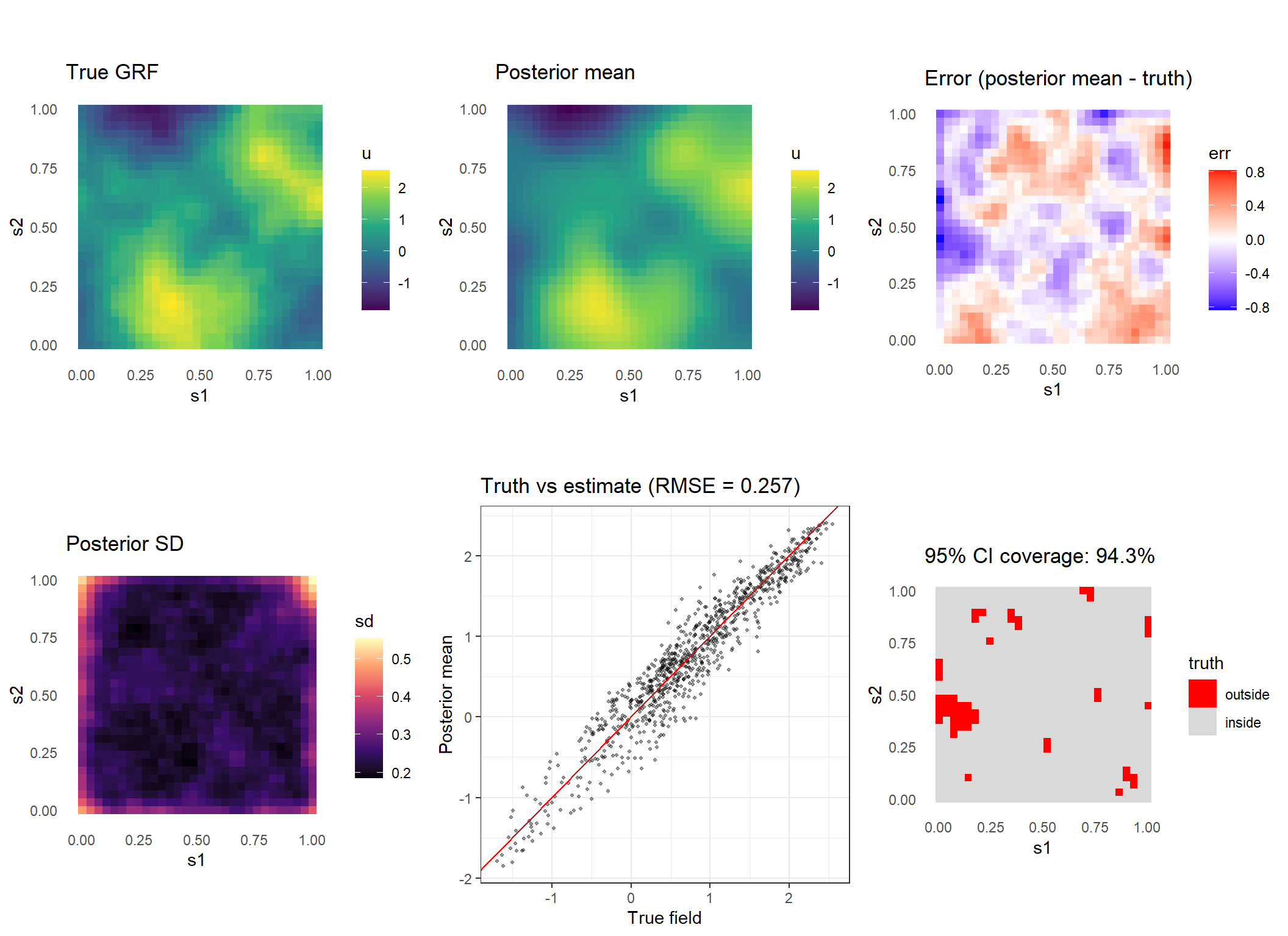
Panels to look at first: the posterior SD should be smallest near observed sites and larger in gaps, and the error map should show no obvious spatial pattern. Because the data come from a Matérn field and the model has a fixed TPS smoothness (\(\nu = 1\)), some systematic mismatch is expected.
7.3 Posterior predictive check
Each posterior draw produces a replicated data set y_sim. We compare the observed data with the replicates through the density overlay, the distribution of the sample mean, and predictive intervals.
y_sim  <- post$y_sim
rep_id <- sample(nrow(y_sim), 100)

ppc_theme <- theme_bw() +
  theme(axis.title   = element_text(face = "bold", size = 12),
        axis.text    = element_text(face = "bold", size = 12),
        legend.title = element_text(face = "bold", size = 12),
        legend.text  = element_text(size = 12))

bayesplot::ppc_dens_overlay(y = y_obs, yrep = y_sim[rep_id, ]) + ppc_theme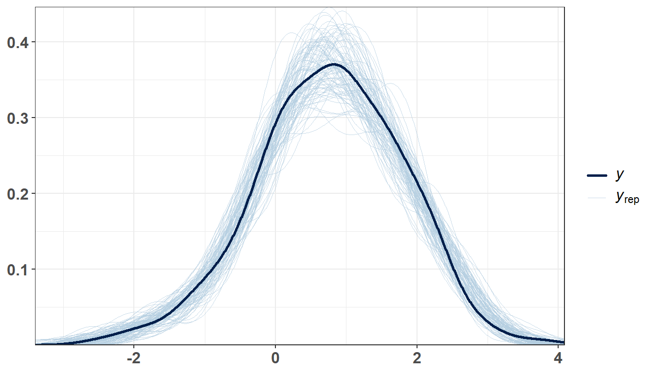
bayesplot::ppc_stat(y = y_obs, yrep = y_sim, stat = "mean") + ppc_theme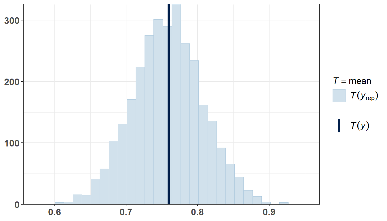
bayesplot::ppc_intervals(y = y_obs, yrep = y_sim[rep_id, ]) + ppc_theme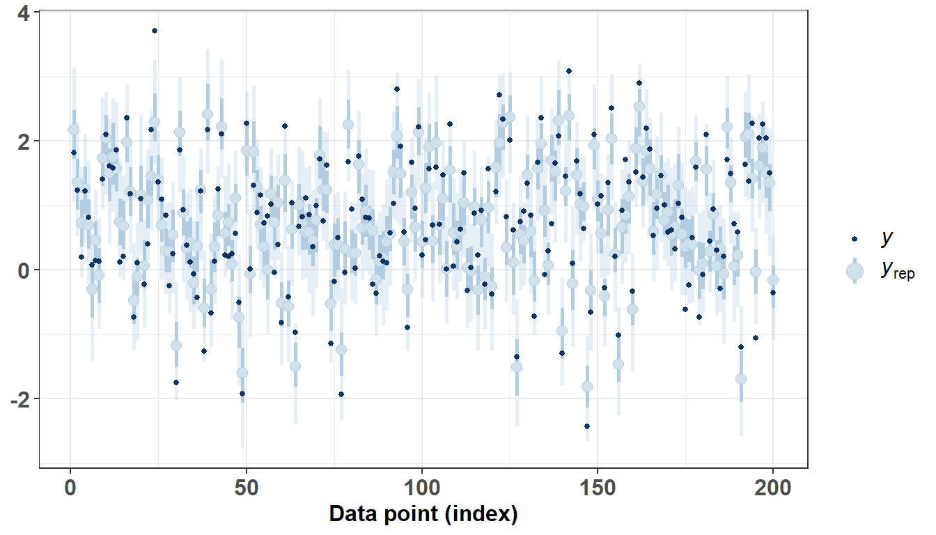
8 Final Comments
In this tutorial we explained the theory of the regTPS approach for Bayesian spatial modeling and showed how to implement it with Stan. The thin plate spline kernel is not a valid covariance function, and regTPS repairs this with the regularized operator \(L_\alpha = \mathbf{I} + \alpha\Delta^2\) to approximate a GRF. In the simulated data with Gaussian error, we recovered the true field and checked the fit with MCMC diagnostics, posterior predictive checks and credible-interval coverage.
The next tutorial will extend this framework to other likelihood functions and to models with additional covariates.
9 References
- Cavieres, J. and Krumscheid, S. regTPS: A novel approach to approximate a Gaussian random field for Bayesian spatial modeling (Statistics and Computing)(Paper).
- Wood, S. N. (2003). Thin plate regression splines. Journal of the Royal Statistical Society B, 65(1), 95-114.
- Wood, S. N. (2017). Generalized Additive Models: An Introduction with R. CRC Press.
- Wahba, G. (1990). Spline Models for Observational Data. SIAM.
- Duchon, J. (1977). Splines minimizing rotation-invariant semi-norms in Sobolev spaces.
- Simpson, D. et al. (2017). Penalising model component complexity. Statistical Science.
- Papaspiliopoulos, O., Roberts, G. and Sköld, M. (2007). A general framework for the parametrization of hierarchical models. Statistical Science.
- Carpenter, B. et al. (2017). Stan: a probabilistic programming language. Journal of Statistical Software, 76(1).